While neural nets are a good way to process data, for tabular data it is quite comon that descision trees work just as well if not better. And they are blazing fast! (Being binary trees and all). Two most common ones are Random Forests and Gradient Boosting Machines. Scary words but simple concepts, really.

Let’s look at them closely.

Let’s set up our notebook first by downloading test data from Kaggle Titanic competition. This a competion to determine a survival probability of a given passenger on Titanic by using data about this passenger (like age, gender, number of children on so on). The data we are downloading is tabular, so fits our goal perfectly. We will try to get to the same accuracy as our previous model with deep learning. First part is setup and downloading test data, so you can skip it:

!pip install kaggle

import os
from pathlib import Path

!mkdir ~/.kaggle
!touch ~/.kaggle/kaggle.json

api_token = {"username":"igornovikov111","key":"df418ab6858712296780fa0800d31ef2"}

import json

with open('/root/.kaggle/kaggle.json', 'w') as file:
 json.dump(api_token, file)

!chmod 600 ~/.kaggle/kaggle.json

import zipfile, kaggle

path = Path('titanic')
if not path.exists():
 kaggle.api.competition_download_cli(str(path))
 zipfile.ZipFile(f'{path}.zip').extractall(path)

from fastai.imports import *
np.set_printoptions(linewidth=130)

Some columns have no values, for whatever reasons, so they have NaN instead. Let’s check how many by summin all NaN values for a all columns:

df = pd.read_csv(path/'train.csv')
tst_df = pd.read_csv(path/'test.csv')

df.isna().sum()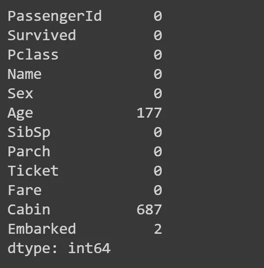

Age and Cabin columns have a lot of NaNs, so we need to work aroun it by replacing those with something. Most common is to replace it with a mode — a most common value in the column. Theres a function mode for that, we take the first row at location 0 (hence iloc[0]).

modes = df.mode().iloc[0]
modes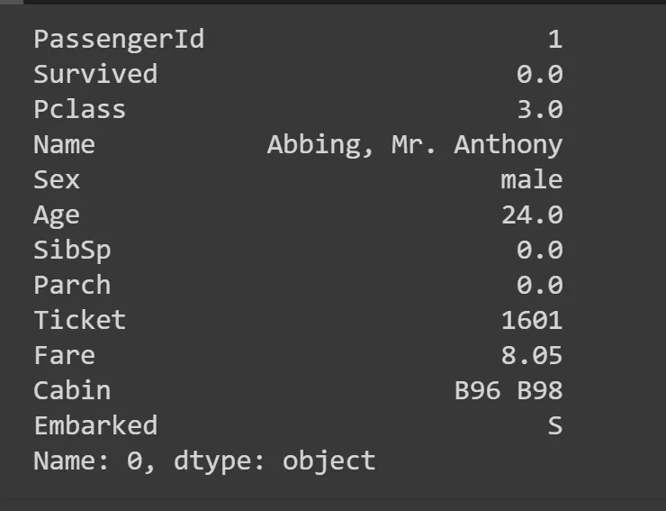

df.fillna(modes, inplace=True)
tst_df.fillna(modes, inplace=True)

Also there are columns that have non-numerical values (sex, embarked). We need to do something about them, so we can split the tree on them. We need to convert them to categorical variables. A categorical variable is a variable that is an index into a list of categories. For gender, for example, the list of categories will be [male, female]. So the value will be 0 (means category at the index 0 at the list) or 1.

df['Embarked'] = pd.Categorical(df.Embarked)
tst_df['Embarked'] = pd.Categorical(tst_df.Embarked)

df['Sex'] = pd.Categorical(df.Sex)
tst_df['Sex]'] = pd.Categorical(tst_df.Sex)

cats=["Sex","Embarked"] # these are categorical column names
conts=['Age', 'SibSp', 'Parch', 'Fare',"Pclass"]

df.Sex.head()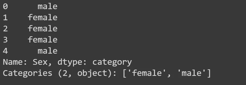

Descision trees and binary splits

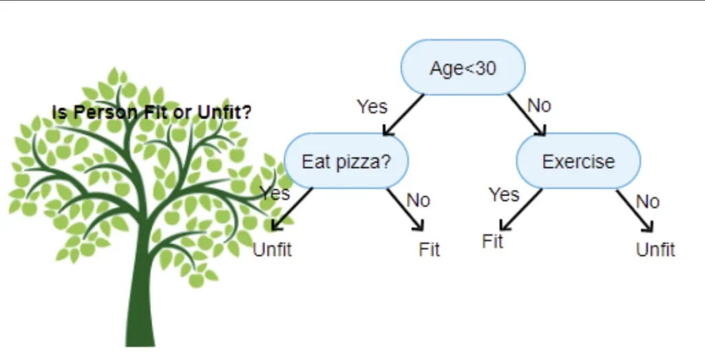
So it has two way splits at each node, called binary split. We can split our set of data 2 ways based on some parameter. For example younger than 30 and older or males and females. We will use a plot to see how that would split up our data — we’ll use the Seaborn library, which is a layer on top of matplotlib that makes some useful charts easier to create.

import seaborn as sns

fig, axs = plt.subplots(1, 2, figsize=(11, 5))
sns.barplot(data=df, y='Survived', x='Sex', ax=axs[0]).set(title="Survival rate")
sns.countplot(data=df, x='Sex', ax=axs[1]).set(title="Gender histogram")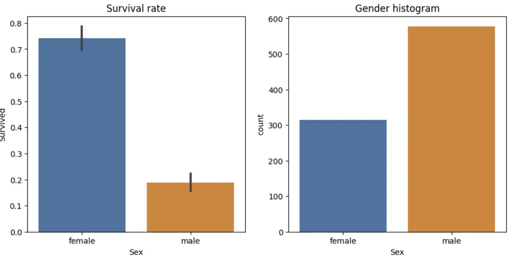

This graph is a good visualization of such a split. A female had way highter chance of survival so it make sense to split this way. So let’s do that. Also we need to set aside part of the date to use later for validation. We will use 25% of all data for that.

from numpy import random
from sklearn.model_selection import train_test_split

random.seed(42)
train_df, val_df = train_test_split(df, test_size=0.25)
train_df[["Sex","Embarked"]] = train_df[["Sex","Embarked"]].apply(lambda x: x.cat.codes)
val_df[cats] = val_df[cats].apply(lambda x: x.cat.codes)

Now let’s create a super simple model that predicts that all females survive and male do not. First we create our in independent variables x (variables we are going to use to predict) and dependent variable y (what we are going to predict).

dep = "Survived"

def xs_y(df):
    xs = df[cats + conts].copy()
    return xs, df[dep] if dep in df else None

train_xs, trn_y = xs_y(train_df)
val_xs, val_y = xs_y(val_df)

display(pd.concat( [train_xs, trn_y], axis=1 ) )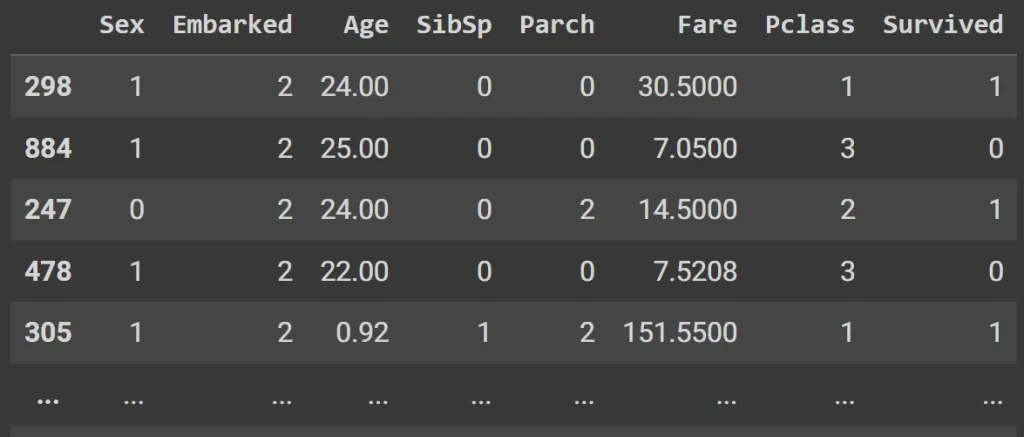

Here is our prediction model set:

preds = val_xs.Sex==0

We are going to use absolute mean error to validate how good is our model:

from sklearn.metrics import mean_absolute_error
mean_absolute_error(val_y, preds)

It will give return something like: 0.21524663677130046.

Alternatively, we can split on a continious column (numerical). For example fare:

df_fare = train_df[train_df.Fare > 0]

figures, axis = plt.subplots(1, 2, figsize=(11, 5))
sns.boxenplot(data=df_fare, x="Survived", y ="Fare", ax=axis[0])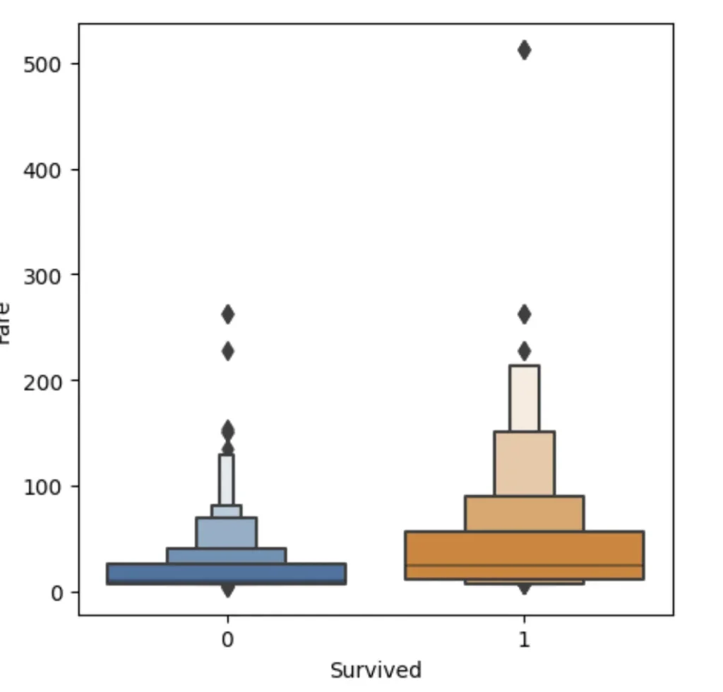

The plots are kinda squashed towards the botton.. Thant’s because there are outliers with very high Fare and to plot them — everything else has to be squashed. We can fix that by taking logarith of Fare instead.

train_df["Fare"] = np.log1p(train_df["Fare"])
val_df["Fare"] = np.log1p(val_df["Fare"])
train_xs, train_y = xs_y(train_df)
val_xs, val_y = xs_y(val_df)

df_fare = train_df[train_df.Fare > 0]

figures, axis = plt.subplots(1, 2, figsize=(11, 5))
sns.boxenplot(data=df_fare, x="Survived", y ="Fare", ax=axis[0])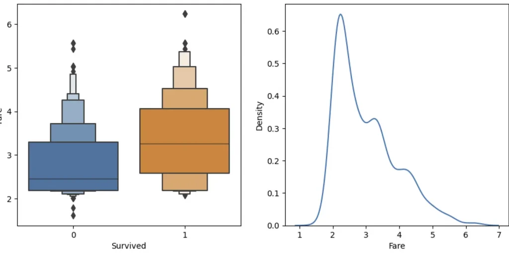

Much better, huh?

The boxenplot shows different quantiles of Fare (well, log of Fare, to be precise) for each group. The wider the group bar, the more people in it. So for example, you can see that most survided people log fare is between 2,5 and 4 (wit average around 3.3) and for not survived average is 2.5. So it seem that people that paid more — survived more often (what a shock!). Anyways, let’s create a simple mode with this observation:

preds = val_xs.Fare>2.5
mean_absolute_error(val_y, preds)

>> 0.3632286995515695

Compare that to our mode using sex — way less accurate. Ideally, we need a way to test dirrerent splits quickly. We will create a function that gives a score for a given split, but this time we are going to use not accuracy bu impurity. Impurity is a mmeasure of how much two groups that a split creates are similar or dissimilar, as that’s what we really want (to create data in two completele different groups).

#convert value of a column base on split value to true or false (we are going to split on that)
split_value = 0.5
lhs = train_xs["Sex"] <= split_value
lhs

# calc the number of rows in first group (with true values)
num_of_rows = lhs.sum()
num_of_rows

>>229

# take all survived values based on the left hand side of a split
train_y[lhs]

Take it’s standart deviation of this set (the dispersion of a dataset relative to its mean. A low standard deviation indicates that the values tend to be close to the mean of the set, while a high standard deviation indicates that the values are spread out over a wider range).

std_deviation = train_y[lhs].std()

And then multiply this by the number of rows in the group, since a bigger group has more impact than a smaller group:

std_deviation * num_of_rows

>> 100.36927432272375

That is our score for that group. Now let’s do a function that calculates that:

def split_score(split, y):
    num_of_rows = split.sum()
    if num_of_rows <=1 : return 0
    return y[split].std()*num_of_rows

def score(col, y, split_value):
    lhs = col<=split_value
    return (split_score(lhs,y) + split_score(~lhs,y))/len(y)

Let’s use our function:

score(train_xs["Sex"], train_y, 0.5)

>> 0.40787530982063946

score(train_xs["Fare"], train_y, 0.5)

>> 0.48282577488540546

As we’ve seen from previous tests — LogFare seems to be a better split. Let’s create a widget where we can dinamically test this:

def iscore(nm, split):
    col = train_xs[nm]
    return score(col, train_y, split)

from ipywidgets import interact
interact(nm=conts, split=15.5)(iscore);

Can we get a computer to automatically calculate an ideal split point for us? To do that for “Age” column we need to create a list of all possible spitl points and than calculete score for each one using our score function and pick one with the lowes score.

col = train_xs["Age"]
unique_set = col.dropna().unique()
unique_set.sort()
unique_set

This is the list of all ages. Let’s find the best one:

calc_point_score = np.vectorize( lambda x: score(col, train_y, x) )

scores = calc_point_score(unique_set)
scores

# let's get the minimum
min_score_index = scores.argmin()
print(min_score_index)
min_point = unique_set[min_score_index]
print(min_point)

So for age the value 6 is the optimal split value. Let’s put this into a function:

def min_col(df, name):
    col, y = df[name], df["Survived"]
    unuque = col.dropna().unique()
    unuque.sort()
    scores = np.array( [score(col, y, x) for x in unuque if not np.isnan(x)] )
    min_score_index = scores.argmin()
    return unuque[min_score_index], scores[min_score_index]

min_col(train_df, "Age")

Let’s try all the columns:

cols = cats+conts
cols

{ x : min_col(train_df, x) for x in cols }

According to this, Sex<=0 is the best split.

How can we improve our model? Let’s take our two groups — male and females and than split each of them too, using different attribute. First, we’ll remove Sex from the list of possible splits (since we’ve already used it), and create our two groups within the split:

if "Sex" in cols: cols.remove("Sex")
display(cols)
ismale = train_df.Sex==1
males, females = train_df[ismale], train_df[~ismale]
males

Now let’s find the single best binary split for males and females:

{x: min_col(males, x) for x in cols}
{x: min_col(females, x) for x in cols}

As we can see the best possible split for males is Age 6, and for females Pclass 2. By chaining these split rules toghether we can create a Descision Tree. Our model first check the gender and based on that will check either Age or Pclass and so on. We’ve done it manually but there is a DecisionTreeClassifier in sklearn.

from sklearn.tree import DecisionTreeClassifier, export_graphviz
m = DecisionTreeClassifier(max_leaf_nodes=4).fit(train_xs, train_y);

One handy feature or this class is that it provides a function for drawing a tree representing the rules:

import graphviz

def draw_tree(t, df, size=10, ratio=0.6, precision=2, **kwargs):
    s=export_graphviz(t, out_file=None, feature_names=df.columns, filled=True, rounded=True,
                      special_characters=True, rotate=False, precision=precision, **kwargs)
    return graphviz.Source(re.sub('Tree {', f'Tree {{ size={size}; ratio={ratio}', s))

draw_tree(m, train_xs, size=10)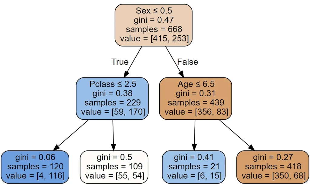

As you can see it found the same split as we did. There is also a new thing called gini. That’s another measure of impurity, very similar to the score() we created earlier. It’s defined as follows:

def gini(cond):
    act = df.loc[cond, dep]
    return 1 - act.mean()**2 - (1-act).mean()**2

What this calculates is the probability that, if you pick two rows from a group, you’ll get the same Survived result each time. If the group is all the same, the probability is 1.0, and 0.0 if they’re all different.

The random forest

With data we have we can’t make a much bigger descision tree. We only have several hundred rows. What if we create several trees, and take the average of their predictions? Taking the average prediction of a bunch of models in this way is known as bagging. Why does that improve the results? We want all models to be uncorellated and trained on different subsets of data. In this case the sum of a lot of uncorrelated errors will average to close to zero.

Here is how we can create different models trained on different subsets of data:

def get_tree(prop=0.75):
    n = len(train_y)
    idxs = random.choice(n, int(n*prop))
    return DecisionTreeClassifier(min_samples_leaf=5).fit(train_xs.iloc[idxs], train_y.iloc[idxs])

trees = [get_tree() for t in range(100)]

Our prediction will be the average of these trees’ predictions:

all_probs = [t.predict(val_xs) for t in trees]
avg_probs = np.stack(all_probs).mean(0)

mean_absolute_error(val_y, avg_probs)

>> 0.22726457399103137

This is almost the same what RandomForestClassifier does, except it also pick a random subset of columns to train each time.

from sklearn.ensemble import RandomForestClassifier

rf = RandomForestClassifier(100, min_samples_leaf=5)
rf.fit(train_xs, train_y);
mean_absolute_error(val_y, rf.predict(val_xs))

0.18834080717488788

One particularly nice feature of random forests and trees is they can tell us which independent variables were the most important in the model, using feature_importances_:

pd.DataFrame(dict(cols=train_xs.columns, imp=m.feature_importances_)).plot('cols', 'imp', 'barh');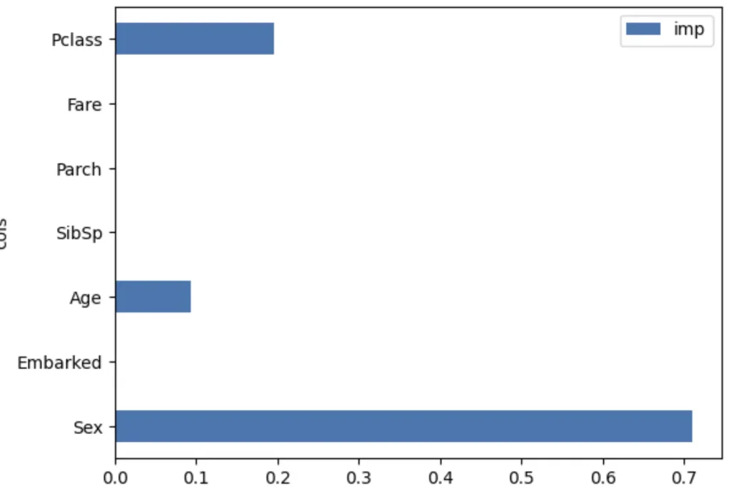

That is it, here it the notebook.